CBSE NCERT Class 12 : Electric Field Lines

We have studied electric field in the last section. It is a vector quantity and can be represented as we represent vectors. Let us try to represent E due to a point charge pictorially. Let the point charge be placed at the origin. Draw vectors pointing along the direction of the electric field with their lengths proportional to the strength of the field at each point. Since the magnitude of electric field at a point decreases inversely as the square of the distance of that point from the charge, the vector gets shorter as one goes away from the origin, always pointing radially outward. In this figure, each arrow indicates the electric field, i.e., the force acting on a unit positive charge, placed at the tail of that arrow. Connect the arrows pointing in one direction and the resulting figure represents a field line. We thus get many field lines, all pointing outwards from the point charge. Have we lost the information about the strength or magnitude of the field now, because it was contained in the length of the arrow? No. Now the magnitude of the field is represented by the density of field lines. E is strong near the charge, so the density of field lines is more near the charge and the lines are closer. Away from the charge, the field gets weaker and the density of field lines is less, resulting in well separated lines. Another person may draw more lines. But the number of lines is not important. In fact, an infinite number of lines can be drawn in any region.It is the relative density of lines in different regions which is important.
      We draw the figure on the plane of paper, i.e., in two dimensions but we live in three-dimensions. So if one wishes to estimate the density of field lines, one has to consider the number of lines per unit cross-sectional area, perpendicular to the lines. Since the electric field decreases as the square of the distance from a point charge and the area enclosing the charge increases as the square of the distance, the number of field lines crossing the enclosing area remains constant, whatever may be the distance of the area from the charge. We started by saying that the field lines carry information about the direction of electric field at different points in space. Having drawn a certain set of field lines, the relative density (i.e., closeness) of the field lines at different points indicates the relative strength of electric field at those points. The field lines crowd where the field is strong and are spaced apart where it is weak. We can imagine two equal and small elements of area placed at points R and S normal to the field lines there. The number of field lines in our picture cutting the area elements is proportional to the magnitude of field at these points. The picture shows that the field at R is stronger than at S. To understand the dependence of the field lines on the area, or rather the solid angle subtended by an area element, let us try to relate the area with the solid angle, a generalization of angle to three dimensions. Recall how a (plane) angle is defined in two-dimensions. Let a small transverse line element dl be placed at a distance r from a point O. Then
the angle subtended by dl at O can be approximated as dq = dl/r. Likewise, in three-dimensions the solid angle* subtended by a small perpendicular plane area dS, at a distance r, can be written as

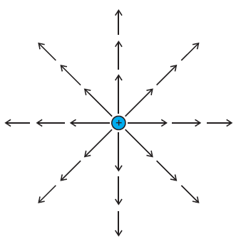
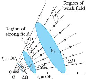dW = dS/r2. We know that in a given solid angle the number of radial field lines is the same. In Fig., for two points P1 and P2 at distances r1 and r2 from the charge, the element of area subtending the solid angle dW is r1^2 dW at P1 and an element of area r2^2 dW at P2, respectively. The number of lines (say n) cutting these area elements are the same. The number of field lines, cutting unit area element is therefore n/( r1^2 dW) at P1 and n/( r2^2 dW) at P2, respectively. Since n and dW are common, the strength of the field clearly has a 1/r2 dependence. The picture of field lines was invented by Faraday to develop an intuitive non- mathematical way of visualizing electric fields around charged configurations. Faraday called them lines of force. This term is somewhat misleading, especially in case of magnetic fields. The more appropriate term is field lines (electric or magnetic) that we have adopted in this book. Electric field lines are thus a way of pictorially mapping the electric field around a configuration of charges. An electric field line is, in general, a curve drawn in such a way that the tangent to it at each point is in the direction of the net field at that point. An arrow on the curve is obviously necessary to specify the direction of electric field from the two possible directions indicated by a tangent to the curve. Field line is a space curve, i.e., a curve in three dimensions. As mentioned earlier, the field lines are in 3-dimensional space, though the figure shows them only in a plane. The field lines of a single positive charge are radially outward while those of a single negative charge are radially inward. The field lines around a system
of two positive charges (q, q) give a vivid pictorial description of their mutual repulsion, while those around the configuration of two equal and opposite charges (q, –q), a dipole, show clearly the mutual attraction between the charges. The field lines follow some important general properties:
(i) Field lines start from positive charges and end at negative charges. If there is a single charge, they may start or end at infinity.
(ii) In a charge-free region, electric field lines can be taken to be continuous curves without any breaks.
(iii) Two field lines can never cross each other. (If they did, the field at the point of intersection will not have a unique direction, which is absurd.)
(iv) Electrostatic field lines do not form any closed loops. This follows from the conservative nature of electric field.