CBSE NCERT Class 12 : Gauss's Law

     As a simple application of the notion of electric flux, let us consider the total flux through a sphere of radius r, which encloses a point charge q at its centre. Divide the sphere into small area elements,
   The flux through an area element dS is where we have used Coulomb’s law for the electric field due to a single charge q. The unit vector ˆr is along the radius vector from the center to the area element.Now, since the normal to a sphere at every point is along the radius vector at that point, the area element dS and ˆr have the same direction. Therefore,

since the magnitude of a unit vector is 1. The total flux through the sphere is obtained by adding up flux through all the different area elements:

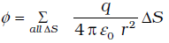
 Since each area element of the sphere is at the same distance r from the charge,

We state Gauss’s law without proof:
Electric flux through a closed surface S

The law implies that the total electric flux through a closed surface is zero if no charge is enclosed by the surface. We can see that explicitly in the simple situation. Here the electric field is uniform and we are considering a closed cylindrical surface, with its axis parallel to the uniform field E. The total
flux f through the surface is f = f1 + f2 + f3, where f1 and f2 represents the flux through the surfaces 1 and 2 (of circular cross-section) of the cylinder and f3 is the flux through the curved cylindrical part of the closed surface. Now the normal to the surface 3 at every point is perpendicular to E, so by definition of flux, f3 = 0. Further, the outward normal to 2 is along E while the outward normal to 1 is opposite to E. Therefore,

where S is the area of circular cross-section. Thus, the total flux is zero, as expected by Gauss’s law. Thus, whenever you find that the net electric flux through a closed surface is zero, we conclude that the total charge contained in the closed surface is zero.
   The great significance of Gauss’s law Eq., is that it is true in general, and not only for the simple cases we have considered above. Let us note some important points regarding this law:
(i) Gauss’s law is true for any closed surface, no matter what its shape or size.
(ii) The term q on the right side of Gauss’s law, Eq., includes the sum of all charges enclosed by the surface. The charges may be located anywhere inside the surface.
(iii) In the situation when the surface is so chosen that there are some charges inside and some outside, the electric field [whose flux appears on the left side of Eq. is due to all the charges, both inside and outside S. The term q on the right side of Gauss’s law, however, represents only the total charge inside S.
(iv) The surface that we choose for the application of Gauss’s law is called the Gaussian surface. You may choose any Gaussian surface and apply Gauss’s law. However, take care not to let the Gaussian surface pass through any discrete charge. This is because electric field due to a system of discrete charges is not well defined at the location of any charge. (As you go close to the charge, the field grows without any bound.) However, the Gaussian surface can pass through a continuous charge distribution.
(v) Gauss’s law is often useful towards a much easier calculation of the electrostatic field when the system has some symmetry. This is facilitated by the choice of a suitable Gaussian surface.
(vi) Finally, Gauss’s law is based on the inverse square dependence on distance contained in the Coulomb’s law. Any violation of Gauss’s law will indicate departure from the inverse square law.

1. Applications of Gauss's Law

The electric field due to a general charge distribution is, as seen above, given by equation. In practice, except for some special cases, the summation (or integration) involved in this equation cannot be carried out to give electric field at every point in space. For some symmetric charge configurations, however, it is possible to obtain the electric field in a simple way using the Gauss’s law. This is best understood by some examples.

1.1 Field due to an infinitely long straight uniformly charged wire

Consider an infinitely long thin straight wire with uniform linear charge density l. The wire is obviously an axis of symmetry. Suppose we take the radial vector from O to P and rotate it around the wire. The points P, P¢, P¢¢ so obtained are completely equivalent with respect to the charged wire. This implies that the electric field must have the same magnitude at these points. The direction of electric field at every point must be radial (outward if l > 0, inward if l < 0). Consider a pair of line elements P1 and P2 of the wire, as shown. The electric fields produced by the two elements of the pair when summed give a resultant electric field which is radial (the components normal to the radial
vector cancel). This is true for any such pair and hence the total field at any point P is radial. Finally, since the wire is infinite, electric field does not depend on the position of P along the length of the wire. In short, the electric field is everywhere radial in the plane cutting the wire normally, and its magnitude depends only on the radial distance r. To calculate the field, imagine a cylindrical
Gaussian surface. Since the field is everywhere radial, flux through the two ends of the cylindrical
Gaussian surface is zero. At the cylindrical part of the surface, E is normal to the surface at every point, and its magnitude is constant, since it depends only on r. The surface area of the curved part is 2(pie)rl, where l is the length of the cylinder.

      Flux through the Gaussian surface
= flux through the curved cylindrical part of the surface
= E × 2(pie)rl

 

 where ˆn is the radial unit vector in the plane normal to the wire passing through the point. E is directed outward if l is positive and inward if l is negative.
    Note that when we write a vector A as a scalar multiplied by a unit vector, i.e., as A = A ˆa , the scalar A is an algebraic number. It can be negative or positive. The direction of A will be the same as that of the unit vector ˆa if A > 0 and opposite to ˆa if A < 0. When we want to restrict to non-negative values, we use the symbol A and call it the modulus of A. Thus, A ³ 0 . Also note that though only the charge enclosed by the surface (ll ) was included above, the electric field E is due to the charge on the entire wire. Further, the assumption that the wire is infinitely long is crucial. Without this assumption, we cannot take E to be normal to the curved part of the cylindrical Gaussian surface. However, equation is approximately true for electric field around the central portions of a long wire, where the end effects may be ignored.

1.2 Field due to a uniformly charged infinite plane sheet

Let s be the uniform surface charge density of an infinite plane sheet. We take the x-axis normal to the given plane. By symmetry, the electric field will not depend on y and z coordinates and its direction at every point must be parallel to the x-direction. We can take the Gaussian surface to be a
rectangular parallelepiped of cross sectional area A, as shown. (A cylindrical surface will also do.) As
seen from the figure, only the two faces 1 and 2 will contribute to the flux; electric field lines are parallel to the other faces and they, therefore, do not contribute to the total flux. The unit vector normal to surface 1 is in –x direction while the unit vector normal to surface 2 is in the +x direction. Therefore, flux E.dS through both the surfaces are equal and add up. Therefore the net flux through the Gaussian surface is 2 EA. The charge enclosed by the closed surface is sA. Therefore by Gauss’s law,

where ˆn is a unit vector normal to the plane and going away from it. E is directed away from the plate if s is positive and toward the plate if s is negative. Note that the above application of the Gauss’ law has brought out an additional fact: E is independent of x also. For a finite large planar sheet, Eq. is approximately true in the middle regions of the planar sheet, away from the ends.

1.3 Field due to a uniformly charged thin spherical shell

Let s be the uniform surface charge density of a thin spherical shell of radius R. The situation has obvious spherical symmetry. The field at any point P, outside or inside, can depend only on r (the radial distance from the centre of the shell to the point) and must be radial (i.e., along the radius vector).

(i) Field outside the shell: Consider a point P outside the shell with radius vector r. To calculate E at P, we take the Gaussian surface to be a sphere of radius r and with centre O, passing through P. All points on this sphere are equivalent
relative to the given charged configuration. (That is what we
mean by spherical symmetry.) The electric field at each point
of the Gaussian surface, therefore, has the same magnitude
E and is along the radius vector at each point. Thus, E and
DS at every point are parallel and the flux through each
element is E DS. Summing over all DS, the flux through the
Gaussian surface is E × 4 pie r^2. The charge enclosed is
s × 4 pie R^2. By Gauss’s law

where q = 4 pie R2 s is the total charge on the spherical shell. Vectorially,

The electric field is directed outward if q > 0 and inward if q < 0. This, however, is exactly the field produced by a charge q placed at the centre O. Thus for points outside the shell, the field due to a uniformly charged shell is as if the entire charge of the shell is concentrated at its centre.(ii) Field inside the shell: In figure, the point P is inside the shell. The Gaussian surface is again a sphere through P centred at O. The flux through the Gaussian surface, calculated as before, is
E × 4 pie r^2. However, in this case, the Gaussian surface encloses no charge. Gauss’s law then gives

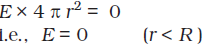
that is, the field due to a uniformly charged thin shell is zero at all points inside the shell. This important result is a direct consequence of Gauss’s law which follows from Coulomb’s law. The experimental verification of this result confirms the 1/r^2 dependence in Coulomb’s law.

Read More

CBSE NCERT Class 12 : Electric Field Lines

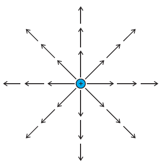
We have studied electric field in the last section. It is a vector quantity and can be represented as we represent vectors. Let us try to represent E due to a point charge pictorially. Let the point charge be placed at the origin. Draw vectors pointing along the direction of the electric field with their lengths proportional to the strength of the field at each point. Since the magnitude of electric field at a point decreases inversely as the square of the distance of that point from the charge, the vector gets shorter as one goes away from the origin, always pointing radially outward. In this figure, each arrow indicates the electric field, i.e., the force acting on a unit positive charge, placed at the tail of that arrow. Connect the arrows pointing in one direction and the resulting figure represents a field line. We thus get many field lines, all pointing outwards from the point charge. Have we lost the information about the strength or magnitude of the field now, because it was contained in the length of the arrow? No. Now the magnitude of the field is represented by the density of field lines. E is strong near the charge, so the density of field lines is more near the charge and the lines are closer. Away from the charge, the field gets weaker and the density of field lines is less, resulting in well separated lines. Another person may draw more lines. But the number of lines is not important. In fact, an infinite number of lines can be drawn in any region.It is the relative density of lines in different regions which is important.
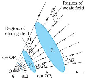
      We draw the figure on the plane of paper, i.e., in two dimensions but we live in three-dimensions. So if one wishes to estimate the density of field lines, one has to consider the number of lines per unit cross-sectional area, perpendicular to the lines. Since the electric field decreases as the square of the distance from a point charge and the area enclosing the charge increases as the square of the distance, the number of field lines crossing the enclosing area remains constant, whatever may be the distance of the area from the charge. We started by saying that the field lines carry information about the direction of electric field at different points in space. Having drawn a certain set of field lines, the relative density (i.e., closeness) of the field lines at different points indicates the relative strength of electric field at those points. The field lines crowd where the field is strong and are spaced apart where it is weak. We can imagine two equal and small elements of area placed at points R and S normal to the field lines there. The number of field lines in our picture cutting the area elements is proportional to the magnitude of field at these points. The picture shows that the field at R is stronger than at S. To understand the dependence of the field lines on the area, or rather the solid angle subtended by an area element, let us try to relate the area with the solid angle, a generalization of angle to three dimensions. Recall how a (plane) angle is defined in two-dimensions. Let a small transverse line element dl be placed at a distance r from a point O. Then
the angle subtended by dl at O can be approximated as dq = dl/r. Likewise, in three-dimensions the solid angle* subtended by a small perpendicular plane area dS, at a distance r, can be written as

dW = dS/r2. We know that in a given solid angle the number of radial field lines is the same. In Fig., for two points P1 and P2 at distances r1 and r2 from the charge, the element of area subtending the solid angle dW is r1^2 dW at P1 and an element of area r2^2 dW at P2, respectively. The number of lines (say n) cutting these area elements are the same. The number of field lines, cutting unit area element is therefore n/( r1^2 dW) at P1 and n/( r2^2 dW) at P2, respectively. Since n and dW are common, the strength of the field clearly has a 1/r2 dependence. The picture of field lines was invented by Faraday to develop an intuitive non- mathematical way of visualizing electric fields around charged configurations. Faraday called them lines of force. This term is somewhat misleading, especially in case of magnetic fields. The more appropriate term is field lines (electric or magnetic) that we have adopted in this book. Electric field lines are thus a way of pictorially mapping the electric field around a configuration of charges. An electric field line is, in general, a curve drawn in such a way that the tangent to it at each point is in the direction of the net field at that point. An arrow on the curve is obviously necessary to specify the direction of electric field from the two possible directions indicated by a tangent to the curve. Field line is a space curve, i.e., a curve in three dimensions. As mentioned earlier, the field lines are in 3-dimensional space, though the figure shows them only in a plane. The field lines of a single positive charge are radially outward while those of a single negative charge are radially inward. The field lines around a system
of two positive charges (q, q) give a vivid pictorial description of their mutual repulsion, while those around the configuration of two equal and opposite charges (q, –q), a dipole, show clearly the mutual attraction between the charges. The field lines follow some important general properties:
(i) Field lines start from positive charges and end at negative charges. If there is a single charge, they may start or end at infinity.
(ii) In a charge-free region, electric field lines can be taken to be continuous curves without any breaks.
(iii) Two field lines can never cross each other. (If they did, the field at the point of intersection will not have a unique direction, which is absurd.)
(iv) Electrostatic field lines do not form any closed loops. This follows from the conservative nature of electric field.

Read More

CBSE NCERT Class 12 : Electric Field

Let us consider a point charge Q placed in vacuum, at the origin O. If we place another point charge q at a point P, where OP = r, then the charge Q will exert a force on q as per Coulomb’s law. We may ask the question: If charge q is removed, then what is left in the surrounding? Is there nothing? If there is nothing at the point P, then how does a force act when we place the charge q at P. In order to answer such questions, the early scientists introduced the concept of field. According to this, we say
that the charge Q produces an electric field everywhere in the surrounding. When another charge q is brought at some point P, the field there acts on it and produces a force. The electric field produced by the charge Q at a point r is given as

where rˆ = r/r, is a unit vector from the origin to the point r. Thus, above equation specifies the value of the electric field for each value of the position vector r. The word “field” signifies how some distributed quantity (which could be a scalar or a vector) varies with position. The effect of the charge
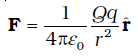
has been incorporated in the existence of the electric field. We obtain the force F exerted by a charge Q on a charge q, as

Note that the charge q also exerts an equal and opposite force on the charge Q. The electrostatic force between the charges Q and q can be looked upon as an interaction between charge q and the electric field of Q and vice versa. If we denote the position of charge q by the vector r, it experiences a force F equal to the charge q multiplied by the electric field E at the location of q. Thus,

The above equation defines the SI unit of electric field as N/C:
(i) From Eq. above, we can infer that if q is unity, the electric field due to a charge Q is numerically equal to the force exerted by it. Thus, the electric field due to a charge Q at a point in space may be defined as the force that a unit positive charge would experience if placed at that point. The charge Q, which is producing the electric field, is called a source charge and the charge q, which tests the effect of a source charge, is called a test charge. Note that the source charge Q must remain at its original location. However, if a charge q is brought at any point around Q, Q itself is bound to experience an electrical force due to q and will tend to move. A way out of this difficulty is to make q negligibly small. The force F is then negligibly small but the ratio F/q is finite and defines the electric field:

A practical way to get around the problem (of keeping Q undisturbed in the presence of q) is to hold Q to its location by unspecified forces! This may look strange but actually this is what happens in practice. When we are considering the electric force on a test charge q due to a charged planar sheet (Section 1.15), the charges on the sheet are held to their locations by the forces due to the unspecified charged constituents inside the sheet.(ii)   Note that the electric field E due to Q, though defined operationally in terms of some test charge q, is independent of q. This is because F is proportional to q, so the ratio F/q does not depend on q. The force F on the charge q due to the charge Q depends on the particular location of charge q which may take any value in the space around the charge Q. Thus, the electric field E due to Q is also dependent on the space coordinate r. For different positions of the charge q all over the space, we get different values of electric field E. The field exists at every point in three-dimensional space.
(iii) For a positive charge, the electric field will be directed radially outwards from the charge. On the other hand, if the source charge is negative, the electric field vector, at each point, points radially inwards.
(iv)   Since the magnitude of the force F on charge q due to charge Q depends only on the distance r of the charge q from charge Q, the magnitude of the electric field E will also depend only on the distance r. Thus at equal distances from the charge Q, the magnitude of its electric field E is same. The magnitude of electric field E due to a point charge is thus same on a sphere with the point charge at its centre; in other words, it has a spherical symmetry.

1. Electric field due to a system of charges

       Consider a system of charges q1, q2, ..., qn with position vectors r1, r2, ..., rn relative to some origin O. Like the electric field at a point in space due to a single charge, electric field at a point in space due to the system of charges is defined to be the force experienced by a unit test charge placed at that point, without disturbing the original positions of charges q1, q2, ...,qn. We can use Coulomb’s law and the superposition principle to determine this field at a point P denoted by position vector r.

    Electric field E1 at r due to q1 at r1 is given by

where 1P ˆr is a unit vector in the direction from q1 to P, and r1P is the distance between q1 and P. In the same manner, electric field E2 at r due to q2 at r2 is

where 2P ˆr is a unit vector in the direction from q2 to P and r2P is the distance between q2 and P. Similar expressions hold good for fields E3, E4, ..., En due to charges q3, q4, ..., qn. By the superposition principle, the electric field E at r due to the system of charges is(as shown in figure):

E(r) = E1 (r) + E2 (r) + … + En(r)

 

E is a vector quantity that varies from one point to another point in space and is determined from the positions of the source charges.

2.Physical significance of electric field

You may wonder why the notion of electric field has been introduced here at all. After all, for any system of charges, the measurable quantity is the force on a charge which can be directly determined using Coulomb’s law and the superposition principle. Why then introduce this intermediate quantity called the electric field? For electrostatics, the concept of electric field is convenient, but not really necessary. Electric field is an elegant way of characterising the electrical environment of a system of charges. Electric field at a point in the space around a system of charges tells you the force a unit positive test charge would experience if placed at that point (without disturbing the system). Electric field is a characteristic of the system of charges and is independent of the test charge that you place at a point to determine the field. The term field in physics generally refers to a quantity that is defined at every point in space and may vary from point to point. Electric field is a vector field, since force is a vector quantity. The true physical significance of the concept of electric field, however, emerges only when we go beyond electrostatics and deal with timedependent electromagnetic phenomena. Suppose we consider the force between two distant charges q1, q2 in accelerated motion. Now the greatest speed with which a signal or information can go from one point to another is c, the speed of light. Thus, the effect of any motion of q1 on q2 cannot arise instantaneously. There will be some time delay between the effect(force on q2) and the cause (motion of q1). It is precisely here that the notion of electric field (strictly, electromagnetic field) is natural and very useful. The field picture is this: the accelerated motion of charge q1 produces electromagnetic waves, which then propagate with the speed c, reach q2 and cause a force on q2. The notion of field elegantly accounts for the time delay. Thus, even though electric and magnetic fields can be detected only by their effects (forces) on charges, they are regarded as physical entities, not merely mathematical constructs. They have an
independent dynamics of their own, i.e., they evolve according to laws of their own. They can also transport energy. Thus, a source of timedependent electromagnetic fields, turned on briefly and switched off, leaves behind propagating electromagnetic fields transporting energy. The concept of field was first introduced by Faraday and is now among the central concepts in physics.

Read More

CBSE NCERT Class 12 : Coulomb’s Law

Coulomb’s law is a quantitative statement about the force between two point charges. When the linear size of charged bodies are much smaller than the distance separating them, the size may be ignored and the charged bodies are treated as point charges. Coulomb measured the force between two point charges and found that it varied inversely as the square of the distance between the charges and was directly proportional to the product of the magnitude of the two charges and acted along the line joining the two charges. Thus, if two point charges q1, q2 are separated by a distance r in vacuum, the magnitude of the force (F) between them is given by

How did Coulomb arrive at this law from his experiments? Coulomb used a torsion balance(A torsion balance is a sensitive device to measure force. It was also used later by Cavendish to measure the very feeble gravitational force between two objects, to verify Newton’s Law of Gravitation.) for measuring the force between two charged metallic spheres. When the separation between two spheres is much larger than the radius of each sphere, the charged spheres may be regarded as point charges. However, the charges on the spheres were unknown, to begin with. Coulomb thought of the following simple way: Suppose the charge on a metallic sphere is q. If the sphere is put in contact with an identical uncharged sphere, the charge will spread over the two spheres. By symmetry, the charge on each sphere will be q/2. Repeating this process, we can get charges q/2, q/4, etc. Coulomb varied the distance for a fixed pair of charges and measured the force for different separations. He then varied the charges in pairs, keeping the distance fixed for each pair. Comparing forces for different pairs of charges at different distances, Coulomb arrived at the relation.

      Coulomb’s law, a simple mathematical statement, was initially experimentally arrived at in the manner described above. While the original experiments established it at a macroscopic scale, it has also been established down to subatomic level (r ~ 10^(–10) m).
      Coulomb discovered his law without knowing the explicit magnitude of the charge. In fact, it is the other way round: Coulomb’s law can now be employed to furnish a definition for a unit of charge. In the relation, k is so far arbitrary. We can choose any positive value of k.The choice of k determines the size of the unit of charge. In SI units, the value of k is about 9×109. The unit of charge that results from this choice is called a coulomb which we defined. Putting this value of k, we see that for
q1 = q2 = 1 C, r = 1 m
F = 9 × 10^9 N
      That is, 1C is the charge that when placed at a distance of 1m from another charge of the same
magnitude in vacuum experiences an electrical force of repulsion of magnitude 9 × 10^9 N. One coulomb is evidently too big a unit to be used. In practice, in electrostatics, one uses smaller units like 1mC or 1μC.
  The constant k is usually put as     for later convenience, so that Coulomb’s law is written as

 

is known as permitivity in free space, its value in SI unit is,8.854 × 10^(–12) C^2 N^(–1)m^(–2)

Since force is a vector, it is better to write Coulomb’s law in the vector notation. Let the position vectors of charges q1 and q2 be r1 and r2 respectively. We denote force on q1 due to q2 by F12 and force on q2 due to q1 by F21. The two point charges q1 and q2 have been numbered 1 and 2 for convenience and the vector leading from 1 to 2 is denoted by r21.

r21 = r2 – r1

In the same way, the vector leading from 2 to 1 is denoted by r12:

r12 = r1 – r2 = – r21
The magnitude of the vectors r21 and r12 is denoted by r21 and r12, respectively (r12 = r21). The
direction of a vector is specified by a unit vector along the vector. To denote the direction from 1 to 2 (or from 2 to 1), we define the unit vectors:

 

Coulomb’s force law between two point charges q1 and q2 located at r1 and r2 is then expressed as

 

 Some remarks on Eq. above are relevant:
• Equation is valid for any sign of q1 and q2 whether positive or negative. If q1 and q2 are of the same sign (either both positive or both negative), F21 is along ˆr 21, which denotes repulsion, as it should be for like charges. If q1 and q2 are of opposite signs, F21 is along –ˆr 21(=ˆr 12), which denotes attraction, as expected for unlike charges. Thus, we do not have to write separate equations for the cases of like and unlike charges. Equation takes care of both cases correctly.
• The force F12 on charge q1 due to charge q2, is obtained from Eq. (1.3), by simply interchanging 1 and 2, i.e.,

Thus, Coulomb’s law agrees with the Newton’s third law.
• Coulomb’s law gives the force between two charges q1 and q2 in vacuum. If the charges are placed in matter or the intervening space has matter, the situation gets complicated due to the presence of charged constituents of matter. We shall consider electrostatics in matter in the next chapter.

 FORCES BETWEEN MULTIPLE CHARGES

The mutual electric force between two charges is given by Coulomb’s law. How to calculate the force on a charge where there are not one but several charges around? Consider a system of n stationary charges q1, q2, q3, ..., qn in vacuum. What is the force on q1 due to q2, q3, ..., qn? Coulomb’s law is not enough to answer this question. Recall that forces of mechanical origin add according to the parallelogram law of addition. Is the same true for forces of electrostatic origin? Experimentally it is verified that force on any charge due to a number of other charges is the vector sum of all the forces on that charge due to the other charges, taken one at a time. The individual forces are unaffected due to the presence of other charges. This is termed as the principle of superposition. To better understand the concept, consider a system of three charges q1, q2 and q3. The force on one charge, say q1, due to two other charges q2, q3 can therefore be obtained by performing a vector addition of the forces due to each one of these charges. Thus, if the force on q1 due to q2 is denoted by F12, F12 is given by even though other charges are present.

In the same way, the force on q1 due to q3, denoted by F13, is given by

which again is the Coulomb force on q1 due to q3, even though other charge q2 is present.
        Thus the total force F1 on q1 due to the two charges q2 and q3 is given as

      The above calculation of force can be generalised to a system of charges more than three. The principle of superposition says that in a system of charges q1, q2, ..., qn, the force on q1 due to q2 is the same as given by Coulomb’s law, i.e., it is unaffected by the presence of the other charges q3, q4, ..., qn. The total force F1 on the charge q1, due to all other charges, is then given by the vector sum of the forces F12, F13, ..., F1n:

The vector sum is obtained as usual by the parallelogram law of addition of vectors.All of electrostats is basically a consequence of Coulomb’s law and the superposition principle.

Read More

CBSE NCERT Class 12 : Electric Charges

1.INTRODUCTION

All of us have the experience of seeing a spark or hearing a crackle when we take off our synthetic clothes or sweater, particularly in dry weather. This is almost inevitable with ladies garments like a polyester saree. Have you ever tried to find any explanation for this phenomenon? Another common example of electric discharge is the lightning that we see in the sky during thunderstorms. We also experience a sensation of an electric shock either while opening the door of a car or holding the iron bar of a bus after sliding from our seat. The reason for these experiences is discharge of electric charges through our body, which were accumulated due to rubbing of insulating surfaces. You might have also heard that this is due to generation of static electricity. This is precisely the topic we are going to discuss in this and the next chapter. Static means anything that does not move or change with time. Electrostatics deals with the study of forces, fields and potentials arising from static charges.

2.ELECTRIC CHARGE

Historically the credit of discovery of the fact that amber rubbed with wool or silk cloth attracts light objects goes to Thales of Miletus, Greece, around 600 BC. The name electricity is coined from the Greek word elektron meaning amber. Many such pairs of materials were known which on rubbing could attract light objects like straw, pith balls and bits of papers. You can perform the following activity at home to experience such an effect. Cut out long thin strips of white paper and lightly iron them. Take them near a TV screen or computer monitor. You will see that the strips get attracted to the screen. In fact they remain stuck to the screen for a while. It was observed that if two glass rods rubbed with wool or silk cloth are brought close to each other, they repel each other. The two strands of wool or two pieces of silk cloth, with which the rods were rubbed, also repel each other. However, the glass rod and wool attracted each other. Similarly, two plastic rods rubbed with cat’s fur repelled each other but attracted the fur. On the other hand, the plastic rod attracts the glass rod and repel the silk or wool with which the glass rod is rubbed. The glass rod repels the fur. If a plastic rod rubbed with fur is made to touch two small pith balls (now-a-days we can use polystyrene balls) suspended by silk or nylon thread, then the balls repel each other and are also repelled by the rod. A similar effect is found if the pith balls are touched with a glass rod rubbed with silk. A dramatic observation is that a pith ball touched with glass rod attracts another pith ball touched with plastic rod These seemingly simple facts were established from years of efforts and careful experiments and their analyses. It was concluded, after many careful studies by different scientists, that there were only two kinds of an entity which is called the electric charge. We say that the bodies like glass or plastic rods, silk, fur and pith balls are electrified. They acquire an electric charge on rubbing. The experiments on pith balls suggested that there are two kinds of electrification and we find that (i) like charges repel and (ii) unlike charges attract each other. The experiments also demonstrated that the charges are transferred from the rods to the pith balls on contact. It is said that the pith balls are electrified or are charged by contact. The property which differentiates the two kinds of charges is called the polarity of charge. When a glass rod is rubbed with silk, the rod acquires one kind of charge and the silk acquires the second kind of charge. This is true for any pair of objects that are rubbed to be electrified. Now if the electrified glass rod is brought in contact with silk, with which it was rubbed, they no longer attract each other. They also do not attract or repel other light objects as they did on being electrified. Thus, the charges acquired after rubbing are lost when the charged bodies are brought in contact. What can you conclude from these observations? It just tells us that unlike charges acquired by the objects neutralise or nullify each other’s effect. Therefore the charges were named as positive and negative by the American scientist Benjamin Franklin. We know that when we add a positive number to a negative number of the same magnitude, the sum is zero. This might have been the philosophy in naming the charges as positive and negative. By convention, the charge on glass rod or cat’s fur is called positive and that on plastic rod or silk is termed negative. If an object possesses an electric charge, it is said to be electrified or charged. When it has no charge it is said to be neutral. A simple apparatus to detect charge on a body is the gold-leaf electroscope. It consists of a vertical metal rod housed in a box, with two thin gold leaves attached to its bottom end. When a charged object touches the metal knob at the top of the rod, charge flows on to the leaves and they diverge. The degree of divergance is an indicator of the amount of charge. Students can make a simple electroscope as follows: Take a thin aluminium curtain rod with ball ends fitted for hanging the curtain. Cut out a piece of length about 20 cm with the ball at one end and flatten the cut end. Take a large bottle that can hold this rod and a cork which will fit in the opening of the bottle. Make a hole in the cork sufficient to hold the curtain rod snugly. Slide the rod through the hole in the cork with the cut end on the lower side and ball end projecting above the cork. Fold a small, thin aluminium foil (about 6 cm in length) in the middle and attach it to the flattened end of the rod by cellulose tape. This forms the leaves of your electroscope. Fit the cork in the bottle with about 5 cm of the ball end projecting above the cork. A paper scale may be put inside the bottle in advance to measure the separation of leaves. The separation is a rough measure of the amount of charge on the
electroscope.To understand how the electroscope works, use the white paper strips we used for seeing the attraction of charged bodies. Fold the strips into half so that you make a mark of fold. Open the strip and iron it lightly with the mountain fold up. Hold the strip by pinching it at the fold. You would notice that the two halves move apart. This shows that the strip has acquired charge on ironing. When you fold it into half, both the halves have the same charge. Hence they repel each other. The same effect is seen in the leaf electroscope. On charging the curtain rod by touching the ball end with an electrified body, charge is transferred to the curtain rod and the attached aluminium foil. Both the halves of the foil get similar charge and therefore repel each other. The ivergence in the leaves depends on the amount of charge on them. Let us first try to understand why material bodies acquire charge. You know that all matter is made up of atoms and or molecules. Although normally the materials are electrically neutral, they do contain charges; but their charges are exactly balanced. Forces that hold the molecules together, forces that hold atoms together in a solid, the adhesive force of glue, forces associated with surface tension, all are basically electrical in nature, arising from the forces between charged particles. Thus the electric force is all pervasive and it encompasses almost each and every field associated with our life. It is therefore essential that we learn more about such a force. To electrify a neutral body, we need to add or remove one kind of charge. When we say that a body is charged, we always refer to this excess charge or deficit of charge. In solids, some of the electrons, being less tightly bound in the atom, are the charges which are transferred from one body to the other. A body can thus be charged positively by losing some of its electrons. Similarly, a body can be charged negatively by gaining electrons. When we rub a glass rod with silk, some of the electrons from the rod are transferred to the silk cloth. Thus the rod gets positively charged and the silk gets negatively charged. No new charge is created in the process of rubbing. Also the number of electrons, that are transferred, is a very small fraction of the total number of electrons in the material body. Also only the less tightly bound electrons in a material body can be transferred from it to another by rubbing. Therefore, when a body is rubbed with another, the bodies get charged and that is why we have to stick to certain pairs of materials to notice charging on rubbing the bodies.

3.CONDUCTORS AND INSULATORS

       A metal rod held in hand and rubbed with wool will not show any sign of being charged. However, if a metal rod with a wooden or plastic handle is rubbed without touching its metal part, it shows signs of charging. Suppose we connect one end of a copper wire to a neutral pith ball and the other end to a negatively charged plastic rod. We will find that the pith ball acquires a negative charge. If a similar experiment is repeated with a nylon thread or a rubber band, no transfer of charge will take place from the plastic rod to the pith ball. Why does the transfer of charge not take place from the rod to the ball? Some substances readily allow passage of electricity through them, others do not. Those which allow electricity to pass through them easily are called conductors. They have electric charges (electrons) that are comparatively free to move inside the material. Metals, human and animal bodies and earth are conductors. Most of the non-metals like glass, porcelain, plastic, nylon, wood offer high resistance to the passage of electricity through them. They are called insulators. Most substances fall into one of the two classes stated above*. When some charge is transferred to a conductor, it readily gets distributed over the entire surface of the conductor. In contrast, if some charge is put on an insulator, it stays at the same place. You will learn why this happens in the next chapter. This property of the materials tells you why a nylon or plastic comb gets electrified on combing dry hair or on rubbing, but a metal article like spoon does not. The charges on metal leak through our body to the ground as both are conductors of electricity.

           When we bring a charged body in contact with the earth, all the excess charge on the body disappears by causing a momentary current to pass to the ground through the connecting conductor (such as our body). This process of sharing the charges with the earth is called grounding or earthing. Earthing provides a safety measure for electrical circuits and appliances. A thick metal plate is buried deep into the earth and thick wires are drawn from this plate; these are used in buildings for the purpose of earthing near the mains supply. The electric wiring in our houses has three wires: live, neutral and earth. The first two carry electric current from the power station and the third is earthed by connecting it to the buried metal plate. Metallic bodies of the electric appliances such as electric iron, refrigerator, TV are connected to the earth wire. When any fault occurs or live wire touches the metallic body, the charge flows to the earth without damaging the appliance and without causing any injury to the humans; this would have otherwise been unavoidable since the human body is a conductor of electricity.

4.CHARGING BY INDUCTION

When we touch a pith ball with an electrified plastic rod, some of the negative charges on the rod are transferred to the pith ball and it also gets charged. Thus the pith ball is charged by contact. It is then repelled by the plastic rod but is attracted by a glass rod which is oppositely  charged. However, why a electrified rod attracts light objects, is a question we have still left unanswered. Let us try to understand what could be happening by performing the following experiment.(i) Bring two metal spheres, A and B, supported on insulating stands, in contact.(ii) Bring a positively charged rod near one of the spheres, say A, taking care that it does not touch the sphere. The free electrons in the spheres are attracted towards the rod. This leaves an excess of positive charge on the rear surface of sphere B. Both kinds of charges are bound in the metal spheres and cannot escape. They, therefore, reside on the surfaces. The left surface of sphere A, has an excess of negative charge and the right surface of sphere B, has an excess of positive charge. However, not all of the electrons in the spheres have accumulated on the left surface of A. As the negative charge
starts building up at the left surface of A, other electrons are repelled by these. In a short time, equilibrium is reached under the action of force of attraction of the rod and the force of repulsion due to the accumulated charges. The process is called induction of charge and happens almost instantly. The accumulated charges remain on the surface, as shown, till the glass rod is held near the sphere. If the rod is removed, the charges are not acted by any outside force and they redistribute to their original neutral state.
(iii) Separate the spheres by a small distance while the glass rod is still held near sphere A. The two spheres are found to be oppositely charged and attract each other.
(iv) Remove the rod. The charges on spheres rearrange themselves. Now, separate the spheres quite apart. The charges on them get uniformly distributed over them. In this process, the metal spheres will each be equal and oppositely charged. This is charging by induction. The positively charged glass rod does not lose any of its charge, contrary to the process of charging by contact. When electrified rods are brought near light objects, a similar effect takes place. The rods induce opposite charges on the near surfaces of the objects and similar charges move to the farther side of the object.

      The centers of the two types of charges are slightly separated. We know that opposite charges attract while similar charges repel. However, the magnitude of force depends on the distance between the charges and in this case the force of attraction over-weighs the force of repulsion. As a result the particles like bits of paper or pith balls, being light, are pulled towards the rods.

Read More

PHY-112 Electricity, Magnetism, and Waves

Introduction
This course covers advances in physics through the 19th century including electromagnetism, optics, and
wave physics. These may seem like separate subjects, but they are related since they both involve the
physics of the continuum, in contrast to the physics of particles covered in Physics 111. Waves involve
continuum physics, while electromagnetism describes the interaction of electromagnetic fields (continuum)
with electric charges (particles). Furthermore, light is simply an electromagnetic wave. It is impossible to
stress the importance of electrodynamics. I will be designing this course to be very interactive so that we
can concentrate on the areas where you are having the most difficulty. It is most important for you to tell
me what you don’t understand so that I can help you figure it out before an exam.
There are four learning goals for this course:
1. Internalize a correct conceptual understanding of key ideas in electromagnetism, optics,
and wave physics.
2. Correctly apply this conceptual understanding to a number of quantitative problems.
3. Connect these concepts to hands-on experience in the lab.
4. Connect these concepts to ideas and models in your primary field of interest.
Learning Physics
The course consists of three class discussions plus a three-hour lab period each week. However, most of the
work in learning physics happens outside of the classroom. Experience has shown that there are a number of
steps you should follow in order to learn new concepts in physics. These are shown in the Physics Learning
Circle. I have designed this course to help you navigate through this learning procedure.

Read
Textbook
Attempt
Workbook
Reading
Quiz
Class
Discussion
Correct
Workbook
Attempt
Homework
Re-read
Textbook
Finish
Homework
Physics
Learning
Circle
Read Textbook
Most of the reading will come from the Knight book this semester. However, if you are interested in taking
the MCAT, I recommend buying the Physics for Pre-meds book, too. It provides a nice overview of the key
ideas.
Physics for Scientists and Engineers, (2nd edition), by Randall D. Knight
You will need to purchase the Value Pack version of Volume 3 (Chapters 20-25, ISBN: 0-321-51669-9) and
Volume 4 (Chapters 26-37, ISBN: 0-321-51670-2) that has the StudentWorkbook bundled with the paperback
textbook. Both volumes should be available at the bookstore. In addition, we will be studying material
from Chapter 15 on fluids and elasticity. You should have the material from Chapter 15 from your Physics
111 text (For those that did not take Physics 111 in the Fall 2008 semester, I can provide a copy of this
material).
I>Clicker, (), by
You must purchase an I>Clicker classroom response pad (ISBN: 0-716-77939-0). These will be used every
day in class to monitor attendance and to monitor your understanding of the material.
Physics for Pre-med, Biology, and Allied health students, (1st edition), by George J. Hademenos
This text will serve as a secondary reference for the course. It is a nice guide and covers a couple of topics
that appear on the MCAT that we will not cover in class.
In addition, there will be various other materials that will be presented for the reading assignments. I will
post these on Moodle.
Reading Timeline: You should do the reading the day before the lecture. This will give you
plenty of time to work through the workbook and take the reading quiz. Approximate time
required: 1 hour
Attempt Workbook
The Student Workbook is designed to be a pre-discussion test of your understanding of the material. The
idea is to do the reading and then answer the workbook questions. I know it seems like a lot of un-graded

work, but experience has shown that if you do the extra work, you will have a better understanding of the
physics. In the end, this will make it much easier to do the homework assignments and to prepare for the
exams. You might not get every question prior to class, but you should look through the workbook and
attempt the problems. I will periodically award extra credit to students that have completed the workbook
pages.
Workbook Timeline: The workbook problems should not take more than half an hour. You
should attempt them the before trying the reading quiz.
Moodle Reading Quiz
There will be a reading quiz posted on Moodle a few days before every discussion period. You are responsible
for completing the quiz before the discussion period starts. Due to the way that Moodle functions, if you
do not complete a Reading Quiz on time, you will recieve a zero score and lose access to that quiz for future
study and review.
Class Discussion
The class period will NOT be devoted to lecture! Rather, it will be primarily spent actively discussing
the concepts covered in each reading assignment and analyzing demonstrations. In addition, I will spend
time (about the last 10 minutes or so) working though the example homework problem. This will be an
opportunity for you to ask questions and practice problem solving together as a class. A complete solution
to these problems will be posted on Moodle. The example problem will be posted with the discussion slides,
notes, and homework package for the day. Printing these before coming to lecture will give you space to take
notes. I will often give hints and suggestions about homework problems, so come prepared to take notes!
I>Clickers: You must purchase an I>Clicker for use in classroom discussions. These will be
used as the feedback tool for in-class questions and discussion. You can purchase one at the
bookstore. You will need to follow the registration instructions given on the first day of class.
Your inputs will be recorded both for attendance purposes, as well as for the in-class extra-credit.
Attendance: Attending class is essential. Attendance will be taken every day using the
I>Clicker. You have three “free” absences, though I would appreciate it if you would let me
know you are going to be gone. You will be responsible for all material covered in class. Every
absence after that will be a 3% reduction in your final grade, i.e. if you miss class 5 times, your
best grade in the class will be a 94%.
Extra Credit: Correct answers to the in-class questions will be worth extra credit on the reading
quiz grade. Reading quizzes are typically worth 40 points. Each correct answer recorded by the
clicker in class will be worth 2 points on the reading quiz grade, up to 10 points.
Correct Workbook
After participating in the class discussion, go back and correct any workbook problems you might have missed.
The solutions to the workbook will be posted on Moodle after class so you can check your understanding of
the concepts.
Attempt Homework
There are four primary reasons for the homework assignments:
1. To gain a working understanding of abstract physics concepts by applying them to problems.

2. To develop problem solving skills.
3. To test your understanding of the material. If you have difficulty doing the problems, then you do not
understand the material. WARNING: The converse is not necessarily true!
4. To connect the models and concepts in physics to similar ideas in chemistry, biology, and medicine.
You should review the solution to the example problem prior to starting your homework. This will give you
guidance on how to model the problems, how to appropriately visualize the relevant ideas, work through the
mathematical models, and assess your answers.
Homework Format:
• Homework will be posted on Moodle and will consist of full-page sheets (one problem per
sheet maximum) that must be printed (on white paper) and used to solve the problems.
• Please put your NAME at top of the front page of each homework set. (If you are turning
in an assignment late, put the date you turned it in.)
• Each problem will contain a number of parts, intended to help guide the problem-solving
process. Each part must be completed and clear work must be shown. All drawings and
diagrams must be clean and neatly drawn– use a straight-edge where appropriate.
• Please box your final answer and make certain it has the correct units where appropriate.
• Work should be neat and legible. Points will be deducted for excessively sloppy work.
• Please staple all sheets together.
• Do not mix assignments. Turn them in as separate sets.
Homework Administration: Problem sets will be due at the BEGINNING of each class
period, and they will be graded and returned the following class period.
Late Homework Policy: No late homework will be accepted (with 3 exceptions) It is
essential to keep up with the homework. Physics takes time to learn—you can’t do it all the night
before the exam. Late Exceptions: You may turn in up to three (3) late homeworks during
the course of the semester. If, for whatever reason, you can not turn the homework on time, do
not complete the assignment on time, or whatever, you may turn in the assignment up to one
week after the original due date for full credit. Students who do not use all of their exceptions
will be awarded extra credit at the end of the semester.
Finish Homework
It is vital that you attempt the homework by yourself PRIOR to seeking help from other students or the
QSC. You will have to take the exams individually, so it is in your best interest to try and do as much of
the homework by yourself as you can. If you need help, go first to the textbook and look at the example
problems. You might also look to see if there are similar problems at the end of the chapter. You will learn
more if you try and work things out for yourself.
If you do work with others on the assignment (and/or consult the tutor in the Quantitative Skills Center),
please jot their names on your problem set. However, the written solutions must be your own. Representing
someone else’s work as yours is cheating and will be treated as such.
Homework Timeline: In order to have time to do the reading and workbook for the next class,
you should begin working on your homework immediately after class. That way you should have
plenty of time to finish it. In many cases, you will find that a problem you do not understand
clears up after letting it sit for a night. Approximate time required: 2 hours

Exams
One of the feedback mechanisms for evaluating your learning is the exam. There will be a total of five exams:
3 in-class exams, 1 take-home exam (to be completed on Moodle) and a final exam. The final exam will
consist of the material from the final section (1/4 of the exam) and a comprehensive coverage of the semester
(3/4 of the exam).
Take-home Exam
One of the exams will be completed out of class. This exam will be administered through Moodle and you
will have 50 minutes to complete the exam. It will consist of 20 multiple choice problems. You will be on
the Gentleman’s Rule that you do not work with or talk to anyone else in the class about the content of the
exam. Although the exam will be open-note, open-book, you will have a limited time to complete the exam.
I recommend studying prior to taking the exam and attempting to take it without the use of notes.
In-class Exams
The in-class exams will be closed book/notebook (No equation sheet or formula sheet will be provided
or allowed). The in-class exams will be multiple choice. However, only partial credit will be given for the
correct response. For full credit you must provide your work and reasoning for each problem. Unexcused
absences for any of the exams will lead to a zero exam score. For an absence to be excused, arrangements
must be made in advance with the instructor.
Final Exam
The final exam will be comprehensive and will be styled in a combination of both the take-home and in-class
exams. No equation sheet will be allowed.
Lab
This lab will be a continuation of your experiences in the Physics 111 Lab. In that lab you learned how to
experimentally test models, how to handle uncertainty analysis, and how to keep an accurate lab notebook.
You will be expected to continue using these skills in the Physics 112 Lab. You will need to purchase a lab
notebook, preferably quad-ruled, for taking data in lab. Notebooks will be graded weekly and you will be
responsible for proper uncertainty analysis, when appropriate.
However, there are a number of new techniques that will be the primary focus of this lab. Two of the goals
for this course are to connect the concepts discussed in class to hands-on experience in the lab. We also want
you to make explicit connections between concepts and ideas and models in your primary field of interest.
Both of these aspects will be ephasized in the lab.
There are three new techniques that you will learn in this lab. These experimental techniques are used
frequently by physicists, although they also can apply to all fields of study. They are:
1. creating rough estimates and approximations to sketch out possible experiments;
2. exploring new technology and equipment to understand their inner workings (including calibrating the
equipment); and,
3. judging different curve fits for accuracy and appropriateness against real data.
The first lab that covers each of these ideas will have a more extensive pre-lab reading so you can get some
practice with the new technique. We will emphasize these techiques throughout the semester. Your lab

notebook should contain your thoughts and experiences with each of these techniques. In addition, you will
be expected to relate the techniques used each week to ideas, models, and skills that could be used in your
major field of interest.
Grading
• Course grades will be determined by your total point score as follows:
Reading Quizzes 5%
Laboratory 25%
Homework 25%
1 Take-home exam 5%
3 In-class exams 25% (for all three)
Final Exam 15%
• In addition, To pass this course, all labs must be completed before the final exam, and the
average score of all exams must be > 52% irrespective of your homework and lab scores.
• Your overall course grade is impossible to determine until the end of the semester when all of the points
are counted. If you wish to measure your performance, compare your scores to the class distribution
which will provided after each exam. If your scores are much below the averages, you should consider
getting help. Don’t wait until it’s too late!!
• Anyone who receives 90% of the total points will receive at least an A−, 80% will receive at least a
B−, etc.
Optional: Historical Paper
You have the option of improving your exam grade by writing a five page biographical paper on one of the
scientists that played a role in the discovery and description of the physical concepts covered in class. This
paper is optional, but if it is submitted, the grade on the paper could replace the score from ONE exam
(not including the final exam). Thus, if you feel you have done poorly on an exam, you can submit the
paper and replace the poor exam grade with the paper grade. You must get approval from the instructor
PRIOR to writing the paper on the person selected as well as the source material to be used as references
for writing the paper. The format of the paper is to be at least five single-sided, double spaced pages, using
12 point font, one inch margins, plus title page and bibliography.
Getting Help
The material in this course is more advanced than in Physics 111 so the tutors in the QSC will not be as
helpful. Therefore, the first place to seek help is your instructor—me! Don’t hesitate to stop by my office
during my office hours or send me an email with a question. In addition, if there is sufficient interest, I can
setup a discussion forum on Moodle for this course so that we can have online discussions of troublesome
areas or topics of interest.
Academic Support Services:
Students with disabilities, whether physical, learning, or psychological, who believe they may need accommodations
in this class, are encouraged to contact Academic Support Services as soon as possible to ensure that

such accommodations are implemented in a timely fashion. Please meet with Julia Rosenberg (ext. 6024)
to verify your eligibility for any classroom accommodations and for academic assistance related to your
disability. You may also discuss your disability with the professor if you wish. All discussions will remain
confidential. If you have a hidden or visible disability which may require classroom or test accommodations,
please see me as soon as possible during a scheduled office hour. If you have not already done so, please
visit Academic Support Services (Armory 101) which is responsible for coordinating accommodations and
services for students with disabilities.
Emergency Procedures
In case of a fire, we are to proceed from the classroom out the nearest exit and toward Sparks Center.
This holds for both class and the lab. You should join the instructor and the class at Sparks to make sure
that everyone got out of the building ok. In the event of a severe weather storm, we are to proceed to the
basement and shelter in the basement hallway.

Read More